I’ve spent the last several months interviewing candidates for Senior Data Engineer positions. I’ve seen some outstanding resumes for people that couldn’t answer this foundational question. Explain SCDs and when you would use each one.
For those in the back, Slowly Changing Dimensions (SCD) are a common data warehousing pattern to manage changing dimensional data (e.g. customer or product attributes over time). Databricks Lakeflow Declarative Pipelnes (formerly Delta Live Tables) provides declarative pipelines and managed ingestion (Lakeflow Connect) that make implementing SCD Type 1 and Type 2 straightforward. Below, I’ll explain how to set up SCD Type 1 vs Type 2 in Lakeflow pipelines (with code examples), how Lakeflow Connect “turns on history” via configuration, comparisons to dbt snapshots, key Lakeflow features for historical dimensions, and best practices for real-world use cases.
SCD Type 1 vs. SCD Type 2 in Lakeflow Declarative Pipelines
SCD Type 1 (overwrite) means updates simply overwrite the old values, not my favorite type because, no history is kept. SCD Type 2 (history tracking) preserves prior records by adding new rows for changes, typically with start and end timestamps or a current flag (sometimes all three) to indicate the period a row version was valid. In Lakeflow Spark Declarative Pipelines, you can implement both SCD types declaratively using the built-in AUTO CDC flow API. This API handles change data capture (inserts, updates, deletes) and can maintain history automatically, eliminating the need for manual MERGE logic or custom code [1][2].
To define a Lakeflow pipeline, you typically create a streaming table as the SCD target (a Delta table that Lakeflow writes to continuously). For SCD Type 2, this table’s schema should include the special timeline columns (by default __START_AT and __END_AT) which Lakeflow uses to record the validity interval of each row version [3][4]. The pipeline then uses an AUTO CDC flow to read from a source (which could be a change feed or stream of source data) and apply changes into the target table.
Example – SCD Type 1 vs SCD Type 2 (Python):
from pyspark import pipelines as dp
from pyspark.sql.functions import col, expr

# Define the source CDC stream (e.g., a table of changes)
@dp.view
def source_cdc():
 return spark.readStream.table(”cdc_data.source_table”)

# Create the target streaming table (dimension table)
dp.create_streaming_table(”dim_table”)

# SCD Type 1 pipeline: overwrites old values (no history)
dp.create_auto_cdc_flow(
 target=”dim_table”,
 source=”source_cdc”,
 keys=[”business_key”], # primary key for matching rows
 sequence_by=col(”sequence_num”), # column to order changes (e.g. timestamp or version)
 apply_as_deletes=expr(”operation = ‘DELETE’”), # handle delete events
 apply_as_truncates=expr(”operation = ‘TRUNCATE’”),# handle table reset events (optional)
 except_column_list=[”operation”,”sequence_num”], # exclude metadata columns from target
 stored_as_scd_type=1 # Type 1: no history tracking
)

# SCD Type 2 pipeline: keeps history (new row per change)
dp.create_auto_cdc_flow(
 target=”dim_table”,
 source=”source_cdc”,
 keys=[”business_key”],
 sequence_by=col(”sequence_num”),
 apply_as_deletes=expr(”operation = ‘DELETE’”),
 except_column_list=[”operation”,”sequence_num”],
 stored_as_scd_type=”2” # Type 2: track full history
 # Optionally: track_history_except_column_list=[”non_critical_col”] # exclude some columns from history tracking
)
In this example, the Type 1 flow will upsert changes so that only the latest value for each business_key is kept (older values are overwritten in-place)[5]. The Type 2 flows, by contrast, will append a new version of a row on updates while marking the previous version as expired[6]. The keys parameter defines the primary key of the dimension (ensuring updates match to the correct entity), and sequence_by is a column (like an updated_at, or SystemModstamp timestamp field, or incremental ID) used to order events and handle out-of-order arrivals. Lakeflow automatically uses this sequence to ensure changes apply in the correct order and to set the __START_AT and __END_AT fields for SCD Type 2[7]. In SCD2 mode, the target table will have additional columns; This way each row version “knows” when it became effective and when it was superseded.
In SQL, the same logic can be expressed with the AUTO CDC INTO syntax. For example, an SCD Type 2 flow in SQL might look like:
CREATE OR REFRESH STREAMING TABLE dim_table (
... all your columns ...,
__START_AT TIMESTAMP, __END_AT TIMESTAMP -- timeline columns for SCD2
);
CREATE FLOW demo_flow AS
AUTO CDC INTO dim_table
FROM STREAM(cdc_data.source_table)
KEYS (business_key)
SEQUENCE BY sequence_num
APPLY AS DELETE WHEN operation = “DELETE”
COLUMNS * EXCEPT (operation, sequence_num)
STORED AS SCD TYPE 2
TRACK HISTORY ON * EXCEPT (non_critical_col);
Here STORED AS SCD TYPE 1|2 toggles the SCD mode[8][9]. The TRACK HISTORY clause (optional) is used to specify which columns should trigger a new historical version – for instance, TRACK HISTORY ON * EXCEPT (city) means all column changes create a new version except changes in the city field, which will be treated as Type 1 updates (overwritten in place)[10][11]. This selective history feature is useful for reducing noise – you might only track significant changes (like a customer’s name or address) but not minor or frequently changing attributes (like a last login timestamp)[12]. By default, if you don’t specify TRACK HISTORY, any change in any column (aside from those excluded via COLUMNS * EXCEPT) will produce a new SCD2 row.
Lakeflow pipelines also provide other convenient options. For example, APPLY AS DELETE WHEN ... maps source indicators (like a CDC operation flag) to actual deletes in the dimension[13][14], and APPLY AS TRUNCATE WHEN ... can handle source-reset events by clearing out the target table (this is typically used only in SCD Type 1 scenarios)[15][16]. There’s also IGNORE NULL UPDATES which can be enabled to prevent null fields in incoming data from overwriting existing values – useful when your source emits partial updates with nulls for unchanged fields[17]. All of these are declared in the pipeline code, and Lakeflow takes care of the heavy lifting at runtime (merging changes, ordering events, etc.).
How it works: When an SCD Type 1 flow runs, the target table is kept at the latest state per key – if a row changes, the old value is gone (replaced by the new value). When an SCD Type 2 flow runs, each update produces a new row version in the target and the previous version’s __END_AT is updated to reflect when it was closed. This happens continuously if the pipeline is running in streaming mode (processing changes as they arrive) or in batch mode on each trigger. The Lakeflow engine ensures consistency even if events arrive out of order. In fact, one major benefit of using Lakeflow is that it automatically handles late or out-of-sequence events in CDC streams – you just declare the sequence column, and the pipeline will correctly reorder and apply changes so that the SCD timeline is accurate[1][18]. This relieves the data engineer from writing complex logic to handle such scenarios.
Enabling History Tracking (SCD2) with Lakeflow Connect
Lakeflow Connect refers to Databricks’ managed ingestion pipelines (using Pipeline assets or YAML/JSON pipeline specs) which can pull data from external sources into the Lakehouse. With Lakeflow Connect, you often configure a pipeline by specifying a connection to a source system (e.g. a database, API, or SaaS connector) and a set of tables or objects to ingest. One key setting in these ingestion pipelines is the “history tracking” option – essentially, whether to treat the data as SCD Type 1 or Type 2.
By default, history tracking is off in Lakeflow Connect pipelines, meaning they operate as SCD Type 1 (each update in the source will overwrite the existing record in the target)[19]. If you want to maintain history (SCD Type 2), you simply turn on history tracking in the pipeline configuration. Turning it on tells Databricks to keep old versions of records rather than overwriting them. In practical terms, that means the target Delta table will include the __START_AT and __END_AT fields to indicate the period each record version was active, similar to the Lakeflow pipeline behavior above. When a new update comes from the source, the pipeline will insert a new row in the target and mark the previous row’s end timestamp, instead of an update-in-place[20].
To enable SCD Type 2 in a Lakeflow Connect pipeline, you configure the pipeline specification. This can be done via a YAML (for Databricks Asset Bundles), via the Databricks UI, or in a notebook using the Pipeline API. For example, in a YAML pipeline definition you could include:
resources:
pipelines:
my_ingest_pipeline:
name: “<pipeline_name>”
catalog: “<target_catalog>”
schema: “<target_schema>”
ingestion_definition:
connection_name: “<source_connection>”
objects:
- table:
source_catalog: “<source_db>” # or source details depending on connector
source_schema: “<source_schema>”
source_table: “<source_table>”
destination_catalog: “<target_catalog>”
destination_schema: “<target_schema>”
table_configuration:
scd_type: SCD_TYPE_2 # turn on history tracking (SCD 2)
sequence_by: “<timestamp_column>” # specify the source column to use for ordering versions
In the above config, setting scd_type: SCD_TYPE_2 under table_configuration enables history tracking for that table[21][22]. We also specify a sequence_by column (such as a last_updated timestamp or an incremental version number from the source) – this is crucial for SCD2, as it defines the order of changes and the time span for each version in the target[23]. The pipeline will use that sequence field to populate the __START_AT (the value when a row version starts) and __END_AT (when it ends) columns on the destination table[24]. (If no sequence_by is provided, some connectors might default to using the source’s replication cursor or timestamp if available, but it’s best practice to specify one explicitly.)
SCD Type 1 vs 2 in Connect – Example: By default (SCD1), each pipeline run will apply updates by updating or deleting records so that the destination reflects the latest state only. If a source record changes or is deleted, the target will overwrite or remove that record (no history kept). If we enable SCD Type 2 (history on), the behavior changes: the pipeline will preserve the old records and add new ones for changes, marking old versions as no longer current.
SCD Type 1 (history off): The most recent value overwrites the old value. In this example, when Alice’s favorite color changed to Purple on Jan 2, the pipeline simply updated her existing record in the target. The old color (Red) is lost, and only the new value is kept (as shown above). No time validity columns are needed in SCD1[19].
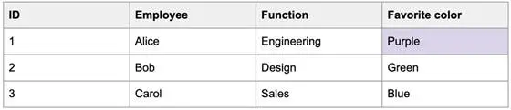
SCD Type 2 (history on): Historical changes are retained. Here, Alice’s original record (Favorite color Red) remains in the table but is marked with an End at of Jan 2, 2025 – indicating it was valid until that date. A new record for Alice (Favorite color Purple) is inserted with a Start at of Jan 2, 2025 and an open End at (null or a placeholder) to denote the current version. The old row is effectively inactive (no longer current) but remains for historical reference[20].

In Lakeflow Connect, enabling SCD2 thus means your target tables will grow vertically (new rows for changes) instead of just updating in place. This is great for audit trails and temporal analysis: you can query the dimension as of any point in time by filtering on the __START_AT/__END_AT range, or easily get the latest record per key by taking the one with __END_AT = NULL (or a special “current” flag if provided).
Technical details and implications: When history tracking is on, the pipeline will not delete data from the target even if it’s deleted in the source – instead, a delete in the source is typically represented as a tombstone row or simply no new updates (the last version remains with a finite end date)[19][20]. This ensures that even deletions can be audited later. Note that not all sources/connectors support SCD Type 2 mode; many do for core tables, but some append-only streams may only support Type 1. For example, Google Analytics 4 connectors support SCD2 on user tables (tracking changes in user profiles over time via last_updated_date), but not on event fact tables which are insert-only[25]. Always check the connector’s feature compatibility to see if SCD2 is available. If it is, Lakeflow Connect makes it as easy as toggling a config flag to get historical dimensions.
On the platform side, turning on history may require a higher-tier pipeline cluster. In fact, the Auto CDC (SCD) features in Lakeflow are supported in Pro or Advanced tiers or in serverless pipelines[26]. This means you should ensure your workspace has the appropriate Lakeflow edition enabled. Also be aware of maintenance: if you ever run a full refresh of a Connect pipeline (reloading an entire table from scratch), it will replace the table and thus wipe out past versions (history starts fresh from the reload point)[27]. This is by design, but it’s a consideration – avoid full refreshes on SCD2 dimensions unless necessary.
Lakeflow vs. dbt Snapshots: Benefits of Databricks-Native SCD
dbt snapshots are a popular way to implement SCD logic (especially Type 2) in a data warehouse. A dbt snapshot typically queries a source table and compares it to the previous run’s state to identify changes, inserting new records for changes or marking old ones as inactive. While effective, this approach requires writing SQL snapshot configurations and scheduling them to run at intervals. Using Databricks Lakehouse native tools (Lakeflow) for SCD offers several advantages for data engineers:
Fully Integrated into Databricks: Lakeflow pipelines run natively on Databricks, using the same engine and Delta Lake features under the hood. There’s no need to manage an external transformation tool or separate orchestration for SCD updates – everything runs in one platform with unified monitoring and governance[28]. (Lineage tracking, data quality checks, and recovery are built-in to Lakeflow pipelines, whereas with dbt you’d rely on separate monitoring or logging.)
Declarative Simplicity (Less Code): Implementing SCD2 in Lakeflow is as simple as adding a parameter or clause (stored_as_scd_type = 2) to your pipeline code[29]. The platform auto-generates the logic to manage history. In contrast, dbt snapshots require you to define the snapshot query, unique keys, and updated-at columns manually. Lakeflow eliminates boilerplate – “hundreds or thousands of lines of manual code” can be reduced to a few lines of declarative config[1]. This reduces the chance of errors in complicated SQL merge logic and lowers maintenance effort.
Streaming and Real-Time Capability: Lakeflow supports streaming CDC pipelines, meaning your dimension table can be kept up-to-date in near real-time as source events arrive[30][31]. This is a big win for use cases that demand fresh data. dbt snapshots, on the other hand, typically run on a schedule (e.g. nightly or hourly) and work on batch snapshots of data. Achieving continuous updates with dbt would require very frequent runs and still wouldn’t truly stream changes as they happen. With Lakeflow, you can have a long-running streaming job that applies changes to the dimension continuously.
Built-in Handling of Out-of-Order and Late Arriving Data: In streaming contexts, events can arrive out of sequence (for example, a late update with an earlier timestamp). Lakeflow’s CDC flows are designed to handle this automatically by using the SEQUENCE BY column to order events and applying a deterministic merge strategy[32]. For SCD Type 2, it even adjusts the __START_AT/__END_AT to maintain correct timelines when events are late. If one tried to implement the same in dbt, it would be quite complex – you’d have to re-run snapshots or have logic to correct out-of-order changes. Lakeflow “sorts it all out without you writing extra logic”[18], which is a significant reliability benefit.
No External Orchestration Needed: A Lakeflow pipeline is a first-class job on Databricks – it automatically handles task scheduling, retries on failures, checkpointing, etc.[33]. With dbt snapshots, you’d typically schedule them via an orchestrator (or cron job) and need to handle failures manually. Databricks pipelines will automatically retry transient failures at the most granular level (task or flow) and ensure exactly-once processing, which reduces operational overhead[33].
Performance and Efficiency: Lakeflow pipelines leverage Delta Lake’s optimized features. For example, if the source is a Delta table with Change Data Feed (CDF) enabled, the AUTO CDC flow can consume just the change feed rather than scanning full datasets[34][35]. This means extremely efficient incremental updates. dbt snapshots often must scan the entire source or do a heavy diff to find changes (unless using an incremental strategy with timestamps). Additionally, Lakeflow’s incremental processing engine for materialized views ensures only new data is processed on each run whenever possible[36], avoiding re-processing the whole dimension. The net result is potentially lower latency and cost.
Advanced Features (Quality, Constraints): Because Lakeflow is a superset of Delta Live Tables, you get extras like data quality enforcement with expectations, auto lineage, and schema evolution handling. For example, you can add an expectation that certain dimension fields are non-null or within ranges, and Lakeflow can drop or quarantine bad records on the fly. dbt has tests which can detect anomalies after the fact, but Lakeflow can enforce them during the pipeline execution.
Unity Catalog & Governance: Lakeflow streaming tables and pipelines integrate with Unity Catalog (Databricks’ governance layer)[37]. This means your SCD dimension table is a managed Delta table in Unity Catalog with all the benefits: fine-grained access control, audit logs, and the ability to discover it via the catalog. dbt’s output tables are also usually in a database, but the integration of governance is tighter in the Lakeflow context.
Of course, there are scenarios where dbt snapshots might be preferable – for instance, if you’re already heavily invested in dbt for transformations and your use case allows batch updates, or if you need a complex custom SCD logic (like Type 3 or Type 6 hybrid) not directly supported by Lakeflow’s built-ins. Lakeflow currently supports only Type 1 and Type 2 out-of-the-box (no native Type 3 or 6)[38], so anything beyond that may require custom coding on Databricks or using dbt. Additionally, Lakeflow’s CDC features require certain Databricks pipeline editions as noted, whereas dbt can run anywhere. But for Databricks-centric architectures, the native SCD capability in Lakeflow offers a simpler, more integrated approach to slowly changing dimensions than maintaining separate dbt snapshot workflows.
Lakeflow Features for Versioned/Historical Dimensions (SCD)
Lakeflow introduces several features that specifically support versioned and historical dimension tables, simplifying SCD workflows and optimizing performance:
AUTO CDC Flows with SCD Modes: The core feature is the AUTO CDC flow type which natively supports SCD Type 1 and Type 2 updates. You simply declare STORED AS SCD TYPE 2 for a flow (or stored_as_scd_type=2 in Python) and Lakeflow will automatically manage the SCD2 mechanics – generating new rows for changes, maintaining pointers to previous versions, and handling all data mutations under the hood[4]. This greatly simplifies implementation: to switch a dimension from Type 1 (no history) to Type 2 (with history) requires just that one config change, with no custom MERGE SQL or additional tables.
Time-Validity Columns (__START_AT, __END_AT): For SCD Type 2 tables, Lakeflow uses two generated timestamp columns to record each row version’s validity interval[3][39]. The pipeline automatically populates these. The current version of a dimension record will have __END_AT = NULL (or a default max date), and when a new update arrives, Lakeflow sets the old row’s __END_AT to the sequence timestamp of the new change. This makes querying historical data straightforward (e.g. you can find what a dimension’s attributes were at a specific time by filtering where that time falls between __START_AT and __END_AT). There’s no need for you to manually manage these timestamps or flags – Lakeflow pipelines take care of it when history tracking is enabled[7].
Partial History Tracking: Lakeflow allows specifying that only certain columns should trigger new historical versions. Using TRACK HISTORY ON * EXCEPT (col1, col2, ...) (or the Python track_history_except_column_list parameter), you can exclude some attributes from history tracking[11]. Changes in excluded columns will be applied as if SCD Type 1 (in-place update), whereas changes in other columns create a new Type 2 version. This feature is useful for high-churn fields that aren’t analytically important to track. For example, you might not want every change in a “last_login_time” to generate a new customer record version. By excluding it, you reduce unnecessary version rows while still tracking substantive changes (like name or address updates) fully[40].
Ignore-Null and Other CDC Options: When working with CDC feeds, it’s common to have sparse updates (only changed fields included, others set to NULL). Lakeflow’s IGNORE NULL UPDATES option (in SQL) instructs the flow to preserve existing values for any columns that come in as NULL in an update[17]. This prevents accidentally wiping out data in the target dimension when the source sends partial changes. Similarly, Lakeflow supports filtering out no-op updates (where data didn’t actually change) so they don’t create new versions. Combined with the except_column_list (which excludes technical columns like sequence numbers or operation flags from being stored), these features optimize the SCD process by focusing only on meaningful changes.
Built-in Delete Handling (Soft Deletes): Lakeflow can manage deletions gracefully in an SCD pipeline. Using APPLY AS DELETE WHEN ..., you define the condition for delete events (for instance, operation = ‘DELETE’ coming from your source CDC feed)[8][41]. In an SCD Type 2 scenario, when a delete event is received, Lakeflow will not actually drop the record from the table; instead it will mark the existing record as ended (just as if an update arrived that superseded it). In other words, deletes become tombstone versions – the record’s __END_AT gets set (and an is_current flag would turn false if using one) to indicate it’s no longer active[42][43]. This ensures the historical record of that entity still exists for audit, but queries for current data can exclude it. (For SCD Type 1, a delete would simply remove the record from the table on the next run.)
Automatic Table Management: The target dimension table in Lakeflow is a managed streaming table. Lakeflow takes care of creating it (with appropriate schema) and can automatically evolve the schema if upstream changes (when using Auto Loader or certain connectors). The pipeline also handles checkpointing so it knows what changes have been applied. All of this means once you configure the SCD pipeline, it reliably maintains the dimension table state without manual intervention. You can also use Delta Lake features on these tables (OPTIMIZE, ZORDER, etc.) as needed – they are just Delta tables under the hood.
Performance Optimizations: Under the declarative approach, Lakeflow optimizes the SCD processing. For example, the incremental materialization ensures only new data is processed each update[36]. The heavy lifting of ordering events and merging is done in Spark but using a declarative plan that Databricks tunes. Because it’s integrated, the engine can do things like task-level retries (retrying only a failed micro-batch rather than the whole job) and intelligent partitioning. This is largely transparent, but it means an SCD pipeline can run continuously without user tuning. Additionally, the separation of flows means you can isolate the dimension processing logic – e.g. one flow per dimension – enabling easier debugging and scaling.
Edition Tiers (Core/Pro/Advanced): Lakeflow pipelines come in tiers; advanced SCD features (Auto CDC flows) require Pro or higher editions[26]. While not a feature per se, it’s worth noting because at higher tiers you also get capabilities like serverless compute for pipelines and faster recovery. The tiered approach allows choosing the right level of capability and cost. For pure batch SCD with small data, one might use a simpler approach (or dbt), but for large-scale or streaming SCD, investing in the higher-tier Lakeflow can pay off with its optimizations and reduced maintenance.
In summary, Lakeflow provides a rich, purpose-built set of features for managing SCD tables. It essentially productizes the SCD pattern: rather than writing bespoke ETL code to handle dimension changes, you declare your intentions (keep history or not, which columns to track, etc.) and let Databricks manage the state. This not only saves development time but also ensures best practices (like correct handling of late data and deletes) are built-in[18][44].
Real-World Use Cases and Best Practices
Lakeflow’s SCD capabilities are being applied in various real-world scenarios. Here are a few common use cases and some best practice tips for data engineers and architects using Databricks:
Customer 360 and Profile History: A typical use case is maintaining a Customer Dimension with full change history for compliance and analytics. For example, consider a retail company syncing customer profiles from a MySQL CRM into the Lakehouse. Using Lakeflow, a streaming CDC feed (via Debezium or the database’s binlog) can land changes into a customers table on Delta. A Lakeflow pipeline can then apply AUTO CDC into a customer_dim streaming table with SCD Type 2 enabled. This ensures that if a customer’s address or preferences change, the old values are preserved as historical records. Analysts can query the customer_dim table to see a customer’s attributes as of any date, or flag the latest record for each customer. This is critical for regulatory needs (e.g., GDPR, where you might need to show what data you had about a customer at a given point in time) and for trend analysis (e.g., how customer segments evolve). Best practice: use a reliable timestamp (e.g., last_updated) from the source as the sequence_by column, and ensure the primary key (customer_id or similar) is used as keys so that each customer’s changes are tracked under the correct identity[45]. Also consider excluding non-essential fields from history (e.g., a “last_login_time” can be excluded if it changes often and isn’t needed for historical analysis) to reduce noise[40].
Product Catalog and Pricing Changes: Another scenario is a Product Dimension where product details (name, category, price, etc.) change over time. SCD Type 2 is useful here to analyze how product pricing or categorization changes impacted sales. Using Lakeflow, you could ingest periodic snapshots of a product catalog (say a daily full extract from an ERP) with the AUTO CDC FROM SNAPSHOT feature – Lakeflow will diff each snapshot against the last to identify changes and apply them as SCD2 updates[46][47]. This avoids writing manual diff logic. Best practice: if using snapshot ingestion, set up the pipeline with AUTO CDC FROM SNAPSHOT in Python, and provide an increasing snapshot version or date as the sequence. This approach will automatically handle inserts, deletes, and updates between snapshots efficiently. If a product description changes, Lakeflow will close out the old version and add a new one with the new description. For querying, you might create a view or use a query filter to always get the current product info (where __END_AT IS NULL), or join on a date to get correct historical pricing.
Financial or HR Data (Compliance Focus): In industries like finance or HR, audit trails are crucial. For example, tracking changes to an Employee Dimension (title, department changes, salary band, etc.) can be implemented with SCD Type 2. Databricks recently added connectors like Workday (for HR data) – using Lakeflow Connect, you can ingest Workday reports and simply turn on SCD Type 2 to keep histories of organizational data[48][49]. Best practice: Pay attention to the sequence column for such data. Workday or other SaaS APIs might not give a natural “last updated” for each record; in those cases, the ingestion pipeline might use the ingestion time or a version number as sequence_by. The sequence needs to be monotonic (ever-increasing per entity) to avoid any ambiguity in the order of changes. If you don’t have a good column, one approach is to use the pipeline’s processing timestamp, but ensure your source extracts are consistent. When querying HR dimensions with SCD2, you can do point-in-time headcount or org structure analysis by joining fact data (like a transaction dated X) to the dimension record that was active on date X (using the Start/End timestamps).
Using Lakeflow Connect for SaaS and Database Sources: Many real-world pipelines start with ingesting data from sources like Salesforce, Google Analytics, Oracle, etc. Lakeflow Connect’s managed connectors allow you to configure SCD tracking easily. For instance, Databricks’ Google Analytics connector can ingest GA4 user data; by default it might be SCD1, but if you add scd_type: SCD_TYPE_2, the pipeline will keep a history of user attribute changes over time[25]. Similarly, a SQL Server connector can pull table data continuously, and by setting scd_type: SCD_TYPE_2 with sequence_by: last_modified, you get a continually updating dimension table with full change history[50][51]. This is far simpler than building a custom ETL with SQL MERGE statements. Best practice: when using connectors, refer to Databricks docs for any connector-specific nuances (some might require enabling CDC at source, etc.). Always specify a sequence_by if the connector supports it, to ensure the pipeline knows how to order changes. Also, monitor the pipeline after initial deployment – Lakeflow pipelines provide a UI showing throughput and any errors. For example, if a schema change happens in the source (new column added), Lakeflow can often handle it (adding the new column to the target table if allowed), but it’s good to be aware of such events.
Optimizing SCD Tables: Over time, SCD Type 2 tables can grow large (since each change adds a row). A best practice is to periodically OPTIMIZE these Delta tables and ZORDER by the business key or date if queries require it. Databricks allows scheduling of maintenance tasks or using auto-optimize features. Also consider partitioning the dimension table by a high-level category (if it’s huge and if appropriate) or clustering by key to keep all versions of an entity together. Lakeflow itself doesn’t automatically optimize the tables, so this is a manual but recommended step for production pipelines to keep performance smooth.
Accessing Current vs Historical Data: It’s common to create two views on top of an SCD2 dimension: one that filters to only current records (e.g., WHERE __END_AT IS NULL) for everyday use, and another that exposes the full history for auditing or temporal queries. This way, downstream users who just want the latest dimension don’t accidentally double-count by joining on all historical versions. With Lakeflow, since the schema and columns are standardized (__START_AT, __END_AT), you can also use Delta Lake’s time travel in combination – though note time travel (as in “AS OF version”) returns the state of the table at a time, which is slightly different from SCD history (which is state within the table). Still, having both SCD tracking and Delta time travel can be powerful: e.g., you could see “as of last month, what did our dimension table think the current record was for each entity”.
Testing and Validation: In any SCD implementation, verifying correctness is important. With Lakeflow, you should test scenarios like: an update arriving late (make sure it correctly updates the prior version’s end time), a delete event (ensure the record is marked ended or removed as expected), and a no-op update (make sure it doesn’t create an extra row if nothing changed). The Databricks documentation provides example data to simulate out-of-order updates and truncates[52][53] – you can use similar techniques to validate your pipeline. Lakeflow’s event log can help debug if something seems off.
Hybrid Approaches: Some organizations use Lakeflow for the core SCD processing and still leverage dbt for modeling downstream. For example, Lakeflow keeps a raw change history table, and then a dbt model might build a simplified dimension or add business-specific logic on top of it. This is valid – Lakeflow ensures the raw data is correct, and dbt can be used to present or augment it. Just be mindful of not duplicating the SCD work in both; it’s often best to let Lakeflow handle the changing aspect, then treat it as just another table in dbt models.
In conclusion, Databricks Lakeflow (including its Connect ingestion pipelines) provides a powerful and streamlined way to manage slowly changing dimensions directly within the Lakehouse environment. By using declarative pipeline constructs, data engineers can enable full change history with minimal code, benefiting from built-in ordering, automatic versioning (__START_AT/__END_AT), and integration with Delta Lake’s performance and reliability features. Compared to traditional methods like hand-rolled MERGE statements or external snapshot tools, Lakeflow’s approach can reduce complexity and improve real-time capabilities[54][55]. For data teams building Dimensional Models on Databricks, leveraging these native SCD features can lead to more maintainable pipelines and trustworthy historical data, all while staying within a unified, governed platform.
Sources:
· Databricks Documentation – Lakeflow Spark Declarative Pipelines and Change Data Capture (AUTO CDC)[1][5][6][7]
· Databricks Documentation – Lakeflow Connect (Managed Ingestion) – History Tracking (SCD Type 2)[19][20][22]
· Databricks Blog/Medium – Real-Time CDC with Lakeflow Pipelines (features and examples of AUTO CDC)[4][12][18]
· SunnyData Blog – Managing SCDs in Databricks (discusses Lakeflow vs. MERGE and when to use each)[29][56]
· Cloudaeon Blog – Simplify Streaming ETL with Lakeflow Pipelines (highlights built-in SCD1/SCD2 and other benefits)[37]
About the Author
Chris Gambill is a data strategy and engineering consultant with over 25 years of experience designing and modernizing data architectures for mid-market and enterprise organizations. As the founder of Gambill Data, he helps businesses bridge the gap between strategy and implementation—building scalable, governed, and AI-ready data ecosystems on platforms like Databricks and Azure.
Chris also runs The Data Engineering Channel on YouTube, where he shares no-fluff insights, frameworks, and tutorials to help data professionals sharpen their skills and stay ahead in a rapidly changing field.